When was the best music made?

I find a ranking of music preferences of critics is from Acclaimed Music, and lists of most sold music from Tsort.

Code

library(jsmp)
library(janitor)

excel_to_tsv <- function(){
  read_excel("files/top_10000_songs_180715.xlsx") |> 
    select(Critic_rank = "PLACE\r\n2018-JUL-15", Artist, Song, Year) |> 
    write_tsv("files/acclaimed_songs.tsv")
  
  read_excel("files/top_3000_albums_180715.xlsx") |> 
    select(Critic_rank = "PLACE\r\n2018-JUL-15", Artist, Album, Year) |> 
    write_tsv("files/acclaimed_albums.tsv")  
}
artist_c <- read_tsv("files/artist_corrections.tsv")
album_c <- read_tsv("files/album_corrections.tsv")
song_c <- read_tsv("files/song_corrections.tsv")
exclude_albums = c("1", "Saturday Night Fever", "The Bodyguard", 
                   "Grease: The Original Soundtrack")
correct_songs <- function(df){
  df |>  mutate(song = stringr::str_replace_all
                 (song, setNames(song_c$old, song_c$new))) |> 
    mutate(song = tools::toTitleCase(as.character(song)))
}
correct_albums <- function(df){
  df |> mutate(album = stringr::str_replace_all
                (album, setNames(album_c$old, album_c$new))) |>
    mutate(album = tools::toTitleCase(as.character(album))) |>
    filter(!album %in% exclude_albums)
}
correct_artists <- function(df){
    df |> mutate(artist = stringr::str_replace_all
                  (artist, setNames(artist_c$old, artist_c$new))) |> 
      mutate(artist = tools::toTitleCase(as.character(artist)))
}
selling_songs <- read_csv("files/selling_songs.csv") |> fix_names() |> 
  select(artist, song = name, public_rank = position) |> 
  correct_artists() |> correct_songs()
acclaimed_songs <- read_tsv("files/acclaimed_songs.tsv") |> fix_names() |> 
  correct_artists() |> correct_songs()
selling_albums <- read.csv("files/selling_albums.csv") |> fix_names() |> 
  select(artist, album = name, year, public_rank = position) |> 
  correct_albums() |> correct_artists()
acclaimed_albums <- read_tsv("files/acclaimed_albums.tsv") |> fix_names() |> 
  correct_albums() |> correct_artists()
genres <- read_delim(delim=";", "files/genres.csv", col_types = cols(.default = "c")) |> fix_names()

high_n <- 7000
get_rank <- function(col) {
  return(log(log(10 + high_n)) - log(log(10 + col)))
}
rankify <- function(df){
  df |> replace_na(list(public_rank=high_n, critic_rank=high_n)) |> 
    mutate(public_value = get_rank(public_rank),
    critic_value = get_rank(critic_rank),
    dif = critic_value - public_value,
    sum = critic_value + public_value) |> 
    naniar::replace_with_na(list(public_rank=high_n, critic_rank=high_n))
}
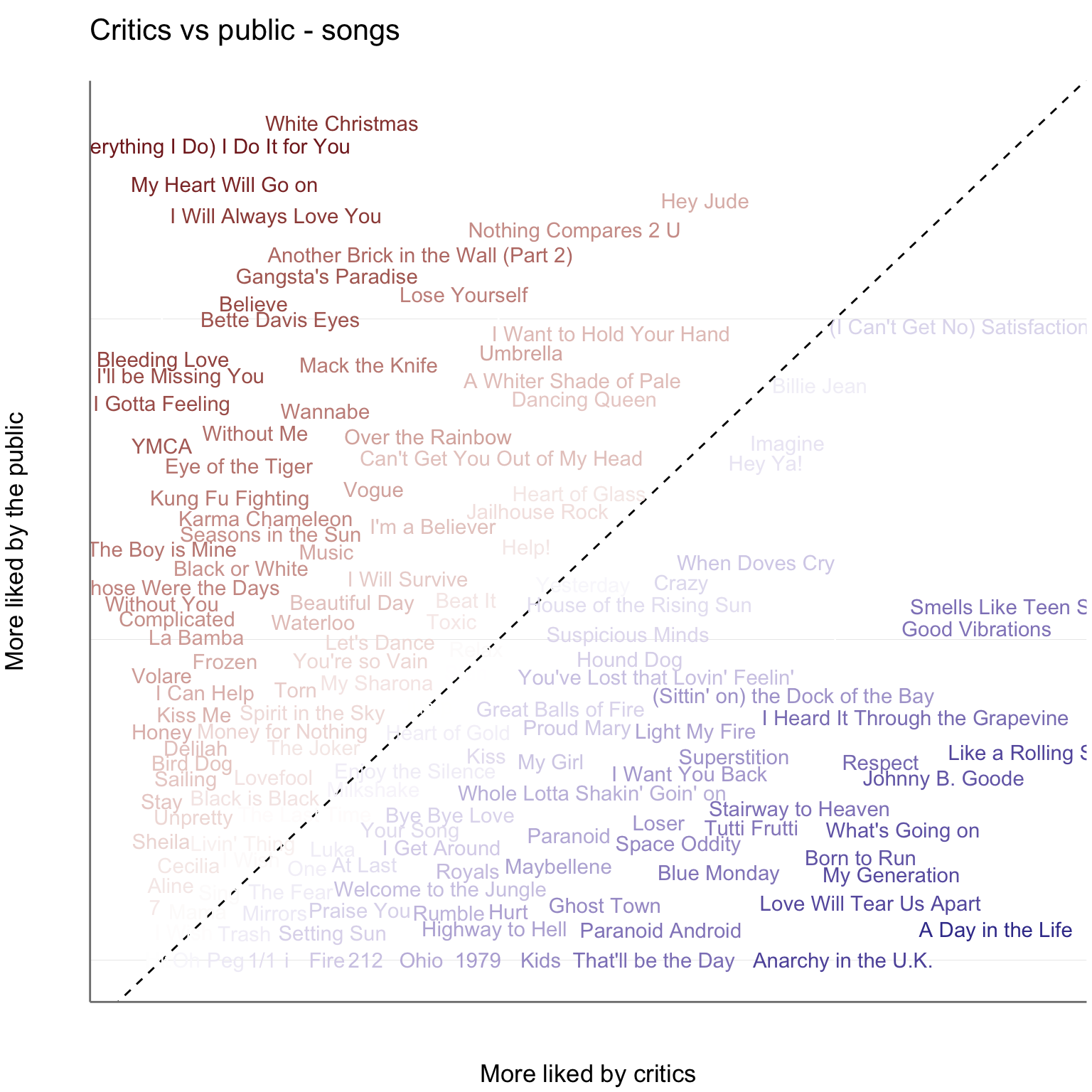
songs = full_join(acclaimed_songs, selling_songs, by=c("artist", "song")) |> rankify()
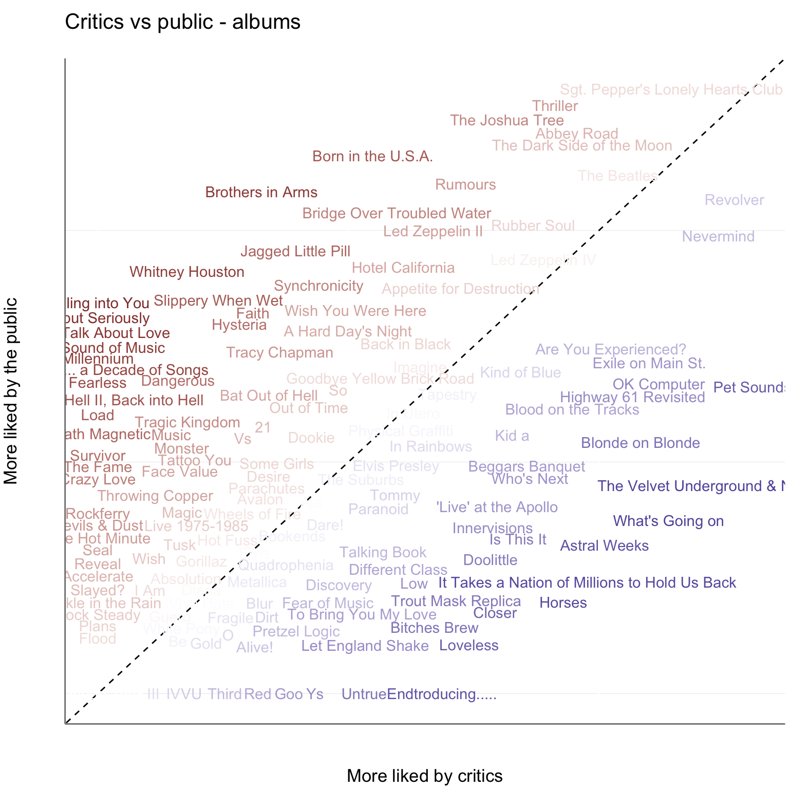
albums = full_join(acclaimed_albums, selling_albums, by=c("artist", "album")) |> rankify()

albums_year <- albums |> mutate(year = year.x) |> group_by(year) |> 
  summarise(acclaim_albums = sum(critic_value))
songs_year <- songs |> group_by(year) |> 
  summarise(acclaim_songs = sum(critic_value))
acclaim <- inner_join(albums_year, songs_year, by="year") |> 
  mutate(acclaim = acclaim_songs + acclaim_albums) |> filter(year > 1949)
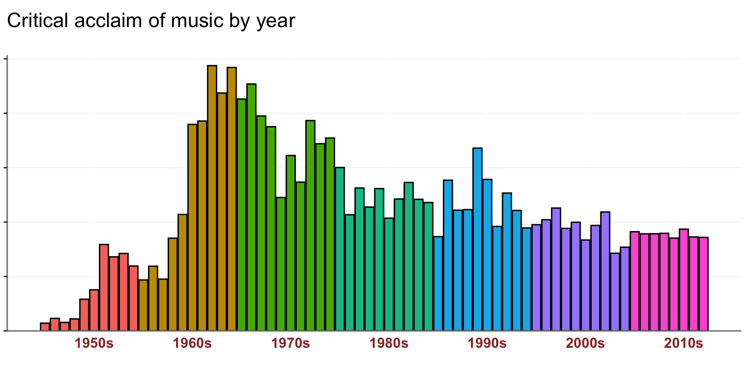
plot_acclaim <- function(df){
  df |> 
    mutate(decade = cut_interval(year, length=10, right=F)) |> 
    ggplot(aes(x = year, y = acclaim, fill=decade, order=decade)) +
      geom_bar(stat="identity") +
      theme(axis.text.x = element_text(face="bold", color="#993333", size=11),
            text = element_text(size=15)) +
      guides(fill=FALSE) + 
      scale_x_continuous(
        breaks=c(1955, 1965, 1975, 1985, 1995, 2005, 2015), 
        labels=c("1950s", "1960s", "1970s", "1980s", "1990s", "2000s", "2010s")) + 
    labs(title = "Critical acclaim of music by year", x = "") +
    gg_y_zero() +
    gg_y_remove()
}

acclaim |> plot_acclaim()

Code

plotg <- function(df, a, b, label, col, title){
  df |> 
    ggplot(aes_string(a, b, label=label, color=col)) +
    geom_abline(intercept=0, slope=1, linetype="dashed") +
    geom_text(check_overlap=T) +
    scale_colour_gradient2(low = muted("red"), high=muted("blue")) + 
    guides(color=F, size=F) +
    theme( 
      axis.title.y = element_text(margin = margin(t = 0, r = 30, b = 0, l = 0)),
      axis.title.x = element_text(margin = margin(t = 30, r = 0, b = 0, l = 0)),
      axis.text.x = element_blank(),
      axis.ticks.x = element_blank(),
      axis.text.y = element_blank(),
      axis.ticks.y = element_blank(),
      axis.title = element_text(size=13)
      ) +
    labs(x = "More liked by critics", y = "More liked by the public",
         title = title)
}

songs |> mutate(dif = critic_value - public_value) |> 
  plotg("critic_value", "public_value", "song", "dif", "Critics vs public - songs")

Code

albums |> mutate(album_dif = critic_value - public_value) |> 
  plotg("critic_value", "public_value", "album", "album_dif", "Critics vs public - albums")

Code

genres2 <- genres |> 
  inner_join(albums, by=c("artist", "album")) |>
  rowwise() |> 
  mutate(
    isRock = "Rock" %in% c(parent1, parent2, parent3),
    isPop = "Pop" %in% c(parent1, parent2, parent3),
    isElectronic = "Electronic" %in% c(parent1, parent2, parent3),
    isRB = "R&B" %in% c(parent1, parent2, parent3),
    isHiphop = "Hip Hop" %in% c(parent1, parent2, parent3),
    isJazz = "Jazz" %in% c(parent1, parent2, parent3)
      )
genres_critics <- genres2 |> 
  group_by(year) |> 
  summarise(
    All = sum(critic_value),
    Rock = sum(critic_value[isRock]) /All,
    Pop = sum(critic_value[isPop]) / All,
    Electronic = sum(critic_value[isElectronic]) / All,
    "R&B" = sum(critic_value[isRB]) / All, All,
    Hiphop = sum(critic_value[isHiphop]) / All,
    Jazz = sum(critic_value[isJazz]) / All)
genres_public <- genres2 |> 
  group_by(year) |> 
  summarise(
    All = sum(public_value),
    Rock = sum(public_value[isRock]) / All,
    Pop = sum(public_value[isPop]) / All,
    Electronic = sum(public_value[isElectronic]) / All,
    "R&B" = sum(public_value[isRB]) / All,
    Hiphop = sum(public_value[isHiphop]) / All,
    Jazz = sum(public_value[isJazz]) / All)

plot_genres <- function(df, title){
  df |> select(-All) |> 
    gather(genre, acclaim, -year) |> 
    filter(year > 1958) |>
    group_by(genre) |> 
    mutate(acclaim = zoo::rollmean(acclaim, 5, na.pad=TRUE)) |> 
    ungroup() |> 
    drop_na() |> 
    ggplot(aes(x=year, y=acclaim, group=genre, color=genre)) + 
      geom_line(size=1.3) +
      scale_x_discrete(breaks = seq(1960, 2010, by = 10)) + 
      theme(axis.text.y = element_blank(),
            axis.text.x = element_text(face="bold", color="#993333", size=12),
            text = element_text(size=18),
            legend.text = element_text(size=15)) +
      labs(x = "Year", title = title)
}

plot_genres(genres_critics, "Critical acclaim of genres over time")

Code

plot_genres(genres_public, "Public popularity of genres over time")